How To Use Decision Models for Evals

📝 摘要 #

决策模型（Decision Models）正在成为 LLM Judge 的低成本替代方案——TypeSafe 的 Jev、Perplexity 的 Decider、Liquid 的 d1、Cloudflare 的 Clef、OpenAI 的 Decisions API 相继出现。本文用 100 条公寓租赁 agent 会话 trace 做二元 pass/fail 评测，对比 Jev 1.13、Perplexity Decider 1.1 27B、Liquid d1 / d1-ultra、Cloudflare Clef Flash 与 OpenAI Decisions（GPT-6 Luna），系统讨论了三个常被忽视的环节：决策阈值调优、性能与成本的帕累托权衡、概率校准。作者指出，直接沿用 API 默认的 0.50 阈值会白白损失大量性能；而原始分数也不能不加验证地当作置信度使用。

核心概念： 决策模型只是分类器，用它们做 eval 必须回到经典分类器评估方法论——先定业务上的 precision/recall 下限，再调阈值，最后才比较成本。

关键技术栈 / 关键要点：

1. 默认阈值陷阱 — 分数分布整体偏低时，0.50 阈值可能一个都抓不到；正确做法是在标注数据上调阈值，并用分层五折交叉验证在训练折选阈值、在验证折测量。
2. 先设业务下限，再优化指标 — 不要盲目最大化 F1。若用于自动告警，应要求 precision 与 recall 同时 ≥ 80%，不达标的模型先淘汰；F-beta 可按业务需要给 precision 或 recall 加权。
3. 性能 vs 成本（帕累托前沿） — 达标候选中，Perplexity 最便宜（0.82 美分 / 100 次评测，F1 0.79），OpenAI Decisions 最高（F1 0.87，3.72 美分，约 4.5 倍成本）。
4. 概率校准 — 0.80 的分数只有在"该分数段的 trace 确实有约 80% 失败"时才可解读为置信度；Platt scaling 显著改善了 Perplexity、Liquid d1 和 Clef Flash，但对 OpenAI 反而略差（Clef Flash 曾出现预测 8% 而实际 60% 失败的严重低估）。
5. 评测范围要窄 — 文中任务刻意宽泛以便拉开模型差距；实践中应针对每种 failure mode 单独建 judge，窄任务下模型间差距会缩小。
6. 决策模型 vs LLM — OpenAI Decisions 底层是 GPT-6 Luna，用最高成本换最高 F1，说明难任务仍可能值得付 LLM 的钱；引用 Randy Olson 的结论：分类与路由可被决策模型替代，需要知识与推理的任务仍需 LLM。

关键结论 / 实践建议： 这是一套迭代流程：调 prompt → 设 precision/recall 下限 → 调阈值 → 查校准 → 权衡成本与延迟，任一环节改动后需重跑后续步骤。作者强调这些并非新方法，而是数据科学家的基本功——"是时候复仇了"。

---

Co-authored with Antaripa Saha.

Decision models have exploded onto the scene recently, starting with TypeSafe’s Jev, followed by Perplexity’s Decider, Liquid’s d1, Cloudflare’s Clef, and OpenAI’s Decisions API. These models promise fast, inexpensive classification.

Decision models are an appealing low-cost alternative to LLM judges for automated evals. But whether they’re the right choice depends on the cost, performance, and latency requirements of your use case.

We’ve also noticed people using the default decision threshold of 0.50 without checking whether it works well for their task. This can leave a lot of performance on the table.

In this post, we’ll start by showing how to tune thresholds to get the best results from decision models. With those thresholds tuned, we’ll compare cost and performance to help you assess which model fits your use case. Finally, we’ll explore how to interpret model scores when deciding whether to act, and how calibration can make them more useful as confidence estimates.

The charts below are static previews. For the best reading experience, I recommend reading this post on hamel.dev, where you can explore the interactive charts.

Read on hamel.dev

What we tested #

We used 100 traces, or logs of conversations and actions, from an apartment leasing agent. The task is to identify traces containing an error, such as a failed booking or a missed handoff to a human. We used the same dataset and broad failure-finding task in our prior post on automated evals. Here, each decision model returns a failure probability for each trace.

We tested Jev 1.13, Perplexity Decider 1.1 27B, Liquid d1 and d1-ultra, Cloudflare Clef Flash, and OpenAI Decisions (GPT-6 Luna). Each model received the same evaluation criteria. The appendix shows the prompt and the structured version used for Jev.

We compare models on two dimensions:

• Performance: We compare each model’s predictions with traces that people have reviewed and labeled as passing or failing. This measures how well the model catches failures while avoiding false alarms.
• Cost: We calculate API cost from token usage and the provider’s prices.

For brevity, we leave latency aside because it depends on factors outside this experiment’s control.

Understanding decision thresholds #

We assign each trace one of two labels, pass or fail. This is a binary pass/fail eval, which we recommend because it encourages clear criteria and is easier to align with human preferences.

Each decision model returns a score from 0 to 1 that estimates how likely a trace is to contain a failure. The APIs turn this score into a decision using a default decision threshold of 0.50. Traces with scores at or above the threshold are flagged as failures. Using this default without checking it against your data can give you subpar results.

For example, a model could assign every failure a score of 0.40 and every passing trace a score of 0.10. Even though this model classifies traces perfectly at a threshold of 0.30, the default threshold of 0.50 would catch nothing.

In practice, scores for failures and passing traces will overlap. Lowering the threshold catches more failures but can also raise more false alarms. Choosing a threshold means balancing:

• Precision: The share of flagged traces that contain a known failure.
• Recall: The share of known failures that the model catches.

The right tradeoff depends on your business goals. For example, criminal trials set a high bar for conviction to avoid convicting innocent people, emphasizing precision. Cancer screening may emphasize recall, accepting more false alarms to miss fewer cases. For this comparison, we’ll give precision and recall equal weight using the F1 score, their harmonic mean. F1 ranges from 0 to 1, and higher is better.

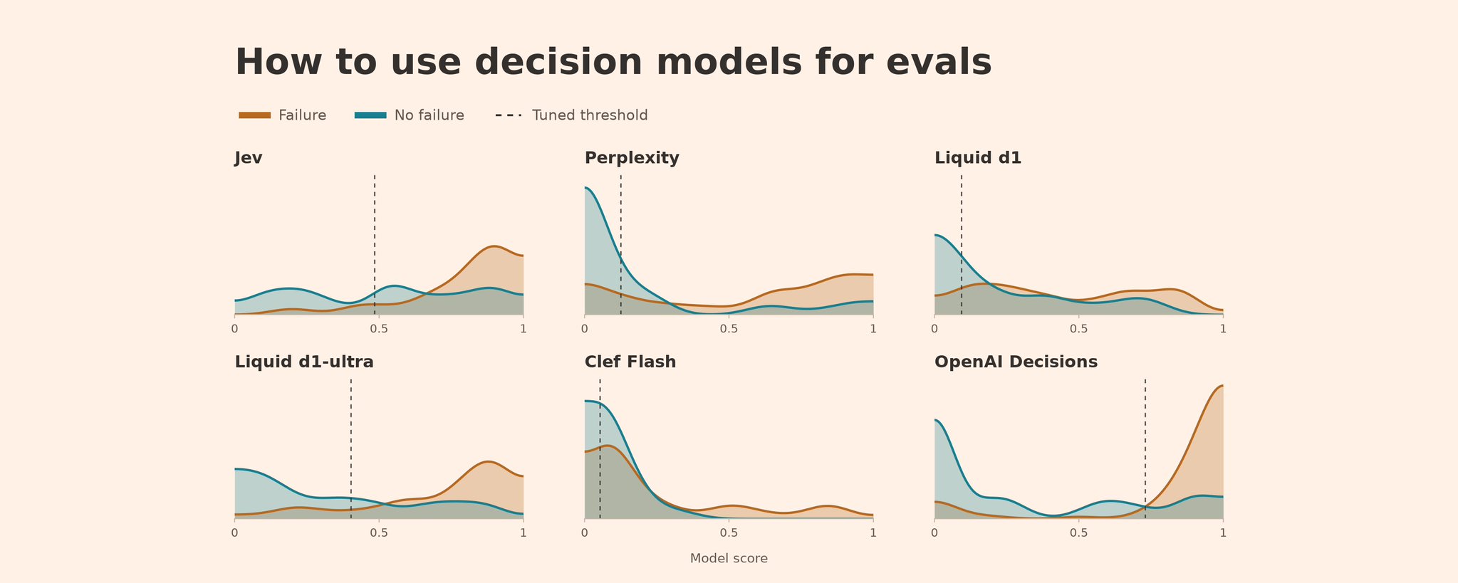
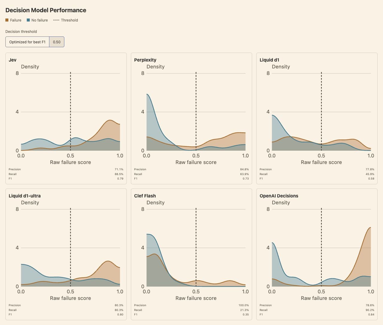
The curves below show how each model scores failures (orange) and passing traces (blue). Taller parts of a curve mean more scores from that class fall in that range. Scores at or above the dashed threshold line are flagged. Use the toggle to compare 0.50 with Optimized for best F1, which chooses a threshold for each model.

Explore the interactive chart on hamel.dev

OpenAI separates the two classes best on this task, which is also reflected in its higher F1 score.

It’s also important not to blindly maximize F1 without thinking about your minimum requirements for the classifier to be useful. For example, if this classifier is used for an automated alerting system, I would want a minimum of 80% on both precision and recall so that I’m minimizing false alarms while catching a sufficient number of failures.

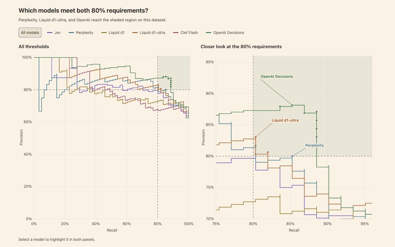
The chart below shows how precision and recall change at different thresholds. The shaded region marks where both reach at least 80%.

Explore the interactive chart on hamel.dev

Perplexity, Liquid d1-ultra, and OpenAI Decisions meet our requirements, but we still need to choose a decision threshold within the shaded region for each model. In the next section, we’ll discuss how to tune those thresholds.

Tuning the decision threshold

For this example, we’ll optimize F1. For our candidates, we’ll restrict tuning to thresholds that meet both 80% minimums on the training data whenever possible. We leave the other models unconstrained to illustrate the effect of tuning.

With labeled traces and saved model scores, you can ask a coding agent to tune the thresholds. Below is an example prompt you can modify for your use case:

Using my saved model scores and binary labels (1 means failure), tune a decision threshold to maximize F1 while requiring at least 80% precision and 80% recall. Use stratified five-fold cross-validation, choosing thresholds on the training examples and measuring performance on the remaining examples. If comparing models, use the same splits for each. Only select thresholds that meet both minimums on the training examples. If none qualifies, report that rather than relaxing either requirement. Report validation precision, recall, and F1, along with any splits where no threshold qualified or validation performance fell below my minimums. Compare with the default threshold of 0.50. Reuse the saved scores without making new model calls.

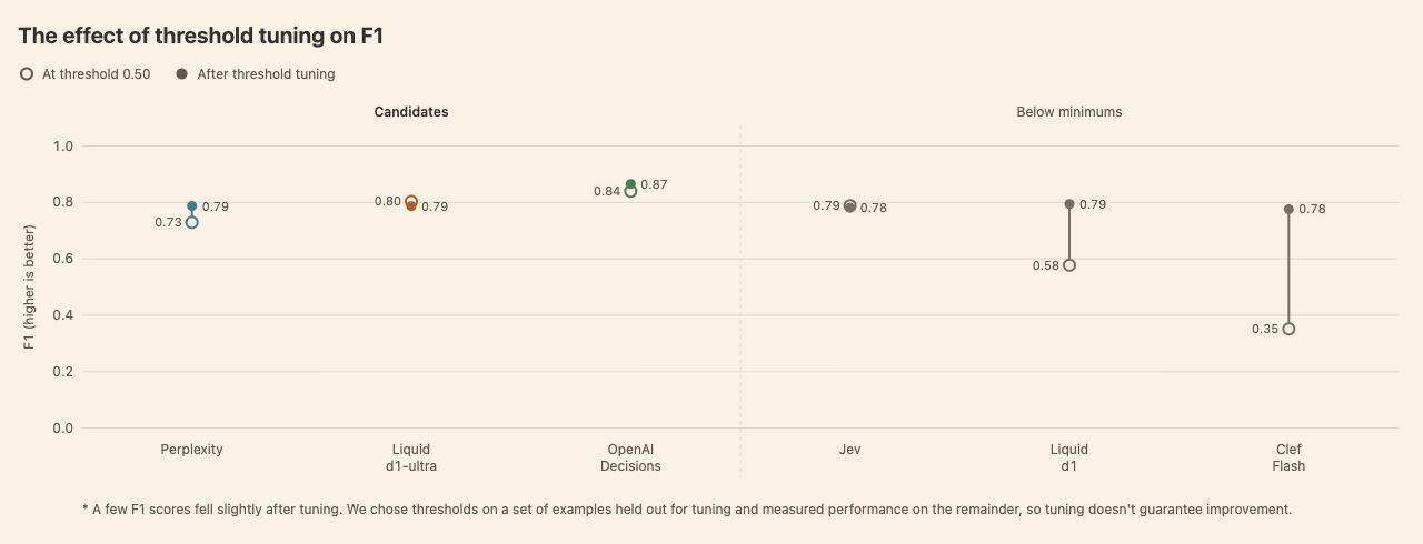
Here’s how tuning for F1 changed each model’s performance. We group the three candidates from the precision-recall chart together and show the other models in gray to illustrate how much tuning can help.

Explore the interactive chart on hamel.dev

Our candidate models gained less from F1 tuning than Liquid d1 and Clef Flash, which fell below our minimums. However, even a small shift in precision and recall can affect business costs or the user experience, so choose the tradeoff deliberately. In practice, it’s unlikely that precision and recall are equally important (as we assumed in this post with F1). For example, the F-beta score lets you give precision more weight with beta below 1, or recall more weight with beta above 1. Optimizing a different metric could lead to different thresholds and results.

Performance versus cost #

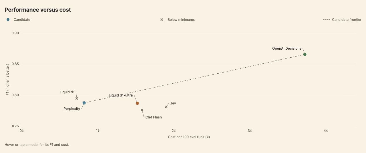
The chart below compares each model’s F1 (after tuning) against cost, focused on our remaining candidates:

Explore the interactive chart on hamel.dev

The dashed line shows the Pareto frontier among our remaining candidates. For any given F1 score, it identifies the cheapest candidate that meets or exceeds that score. This particular chart is a bit silly as there are only three options, but it’s a useful illustration for how to think about cost vs. performance.

Perplexity was the cheapest of these candidates at 0.82 cents per 100 eval runs, with an F1 of 0.79. OpenAI Decisions reached an F1 of 0.87 at 3.72 cents per 100 eval runs, about 4.5 times the cost.

Can we trust the probabilities? #

Beyond pass/fail evals, you may want to use a decision model’s score as a confidence estimate. But can you take that number literally? For a score of 0.80 to mean an 80% chance of failure, roughly 80% of traces with similar scores should contain failures.

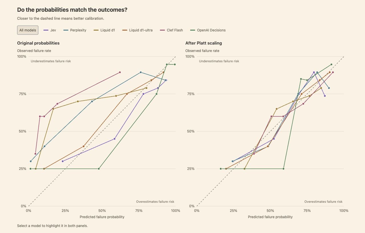
The chart below shows each model’s probability calibration: how closely its predicted probabilities match observed outcomes. Each point represents about 20 traces with similar scores. A point on the diagonal means the predicted probability matches the failure rate in that group. Above the line, the model underestimates the risk of failure. Below it, the model overestimates that risk.

If the predicted probabilities don’t match the observed outcomes, we can adjust them using another model. The second panel shows one method, Platt scaling, which fits a simple curve to make that adjustment.

Explore the interactive chart on hamel.dev

Perplexity, Liquid d1, and Clef Flash move closer to the diagonal after calibration. For example, one group of Clef Flash traces had an average predicted failure probability of about 8%, but 60% contained failures.

Jev and Liquid d1-ultra were already well calibrated on this dataset and needed little adjustment.

Platt scaling isn’t always the best fit. For example, OpenAI’s probabilities got slightly worse with the version of Platt scaling we used. You can direct your coding agent to perform calibration with the following prompt:

Using my saved failure probabilities and binary labels (1 means failure), test whether Platt scaling improves each model’s probabilities. Use stratified five-fold cross-validation with the same splits for every model. Fit the calibration mapping on each training split and apply it to the remaining traces. Fit on log-odds, clipping probabilities away from 0 and 1 first. Plot predicted probabilities against observed failure rates before and after calibration. Report Brier scores (lower is better), and explain which models improved or got worse. Reuse the saved scores without making new model calls.

Prompt tuning and evaluator scope #

We kept the eval task in this post broad to make the differences between models easier to see. In practice, we recommend building a separate judge for each failure mode. With a narrower task and more specific guidance, we expect the performance gaps between models to shrink.

I like to start with a larger model that has acceptable performance on a task and then try smaller models to see if they can match the larger model’s performance for less cost. Prompt tuning can also be helpful if you have high-quality labels. I discuss how to craft a good judge prompt in this post.

Putting these ideas into practice #

For this particular dataset, OpenAI had breakout performance at a higher cost. Perplexity and Liquid d1-ultra offer lower-cost options with lower performance. We have observed that model performance varies substantially across tasks and datasets, which means it’s important to measure things yourself.

To recap:

• Once you’re satisfied with your judge’s prompt, set minimum precision and recall requirements for your use case. Rule out models that cannot meet these.
• Tune each model’s decision threshold before comparing performance. Choose a precision-recall tradeoff that fits your business goals. Be intentional, don’t just use F1 score because this post did!
• If you want to use scores as confidence estimates, check whether the probabilities match observed outcomes. Calibration can help, but you need to measure whether it improves them.
• Weigh performance against cost and latency for your workload.

This process is iterative. You may improve the prompt, then need to tune the threshold again or revisit calibration. In this post, we focused on threshold tuning and calibration because we’ve seen many people use decision models off the shelf without considering these factors.

You might also be wondering how decision models stack up to LLMs. OpenAI Decisions uses GPT-6 Luna, which delivered our highest F1 at the highest cost, suggesting that harder eval tasks may justify paying more for an LLM. In a broader comparison, Randy Olson found that decision models could match LLMs on classification and routing at lower cost, while LLMs pulled ahead on tasks requiring knowledge and reasoning.

None of the ideas discussed in this post are new. Choosing a precision-recall tradeoff, tuning thresholds and comparing performance vs. cost are part of evaluating any classifier. To learn more about these fundamentals, I recommend Machine Learning with Python Cookbook, 2nd Edition by Kyle Gallatin and Chris Albon.

Finally, if you’re a data scientist or ML engineer wondering where you belong in the AI age, these are skills you already have. It’s time to get revenge 🙂.

P.S. I share articles like this and what I’m learning about building AI products in my newsletter. To learn more about evals, Shreya Shankar and I co-authored AI Evals for AI Engineers, published by O’Reilly.

P.P.S. This post has lots of footnotes. You can read them on hamel.dev.