Post-training 101

A hitchhiker's guide into LLM post-training

EP1 of Tokens for Thoughts

Overview

This document serves as a guide to understanding the basics of LLM post-training. It covers the complete journey from pre-training to instruction-tuned models. The guide walks through the entire post-training lifecycle, exploring:

The transition from next-token prediction to instruction following

Supervised Fine-Tuning (SFT) fundamentals, including dataset creation and loss functions

Various Reinforcement Learning techniques (RLHF, RLAIF, RLVR) with detailed explanations of reward models

Evaluation methodologies for assessing model quality

This is our first note and we will discuss post-training intermediate topics next. Please DM us what other topics you would like to learn too. Hope you enjoy!

1. The Journey from Pre‑training to an Instruct‑tuned Model

A base model (or a pre-trained model) is usually created by pre-training on large-scale text and image data [1][2]. The primary goal of pre-training is to encode the world’s (in a narrow sense, the Internet’s) knowledge into the model. The training objective is quite straightforward: the model is trained to predict the next token over many different sequences prior to it [1]. However, while a base model can be very knowledgeable, the training objective of next token prediction also makes it less useful in most applications [3].

The following conceptual comparison (Figure 1) will give you a rough sense of the difference in their behaviors. When prompted with the same question, “What is the capital city of U.S”. Note that here the user prompt does not have a question mark at the end. A pre-trained model (left), which was trained to predict the next token, will firstly predict the question mark (i.e.?) before finishing the rest of the sentence. On the other hand, an instruction-tuned model, will respond “Washington, D.C.” directly, since it was usually trained to answer a user’ question as opposed to continuation [4].

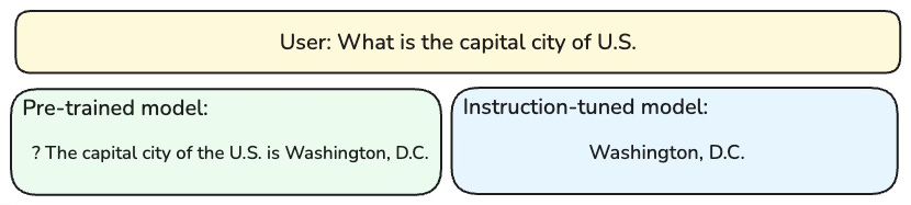
Figure 1. The journey from pre‑training to an instruct‑tuned model.

In order to make the large language model (LLM) actually helpful in answering questions, we usually take a base model and go through post-training (also known as fine-tuning). Instead of using the web corpora crawled from the Internet, post-training data is usually much smaller in size and far more curated [5]. Post-training is used to align model’s behaviors (helpful, honesty, harmless) and improve its capabilities that were accrued from pre-training. There are quite a few popular techniques for post-training, such as supervised fine-tuning (SFT), and reinforcement learning from human feedback (RLHF). After DeepSeek R1 [6], there was an emergence of reinforcement learning with verifiable rewards (RLVR) which is very effective in improving the model’s reasoning and coding capabilities [7].

We will go into more details in the subsequent sections.

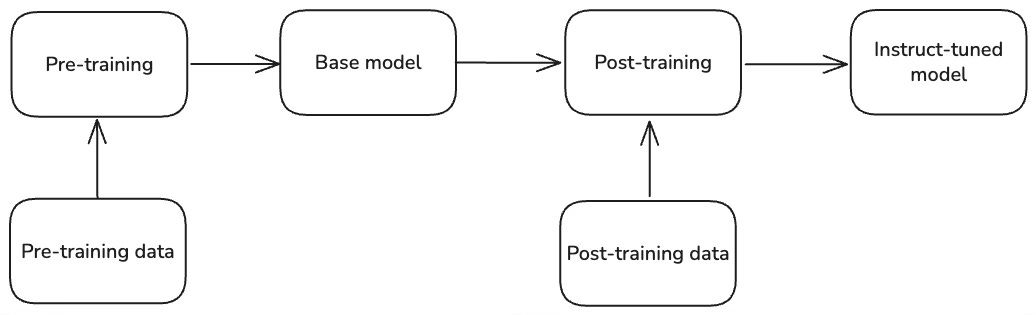
Figure 2. The journey from pre‑training to an instruct‑tuned model.

Sometimes you might also hear about terms like continued pre-training and mid-training. These are somewhat unofficial (or less formal) terms that describe the process of further pre-training a base model over a high-quality dataset and/or a targeted corpora with the goal of improving model’s capabilities in those particular domains. Since pre-training isn’t a focus of this document, we will not go into details here.

2. E2E Life Cycle of Post-training

At a high-level, post-training is the process of taking a base model and turning it into an instruction-tuned model that is both helpful and safe for users (Figure 3). There are usually two main families of training techniques for post-training: supervised fine-tuning (SFT) and reinforcement learning (RL) [4]. At the birth of Instruct-GPT (which is a precursor to GPT-3.5), OpenAI introduced a two-stage process which consisted of SFT and RLHF [3]. In 2024, DeepSeek introduced DeepSeek V3 that heavily used RLVR—VR stands for verifiable rewards (aka rule-based rewards or accuracy rewards) [8]. Later on DeepSeek rolled out the R1 model. It described R1-zero with RL directly on the base model and the final R1 model which employed a two-stage RL- (1) reasoning-oriented RL, then (2) RL “for all scenarios” (alignment with human preferences) [6]. Post-training research is still fast-evolving—usually the so-called best practices become obsolete as the research community continue to make progress in this domain.

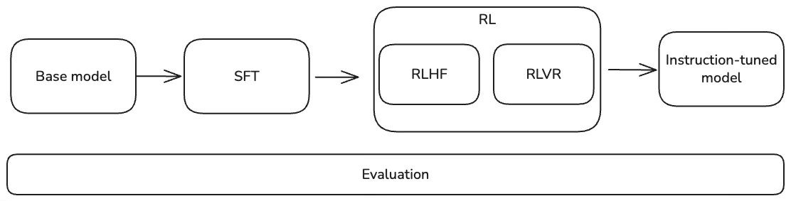
Figure 3. E2E Life Cycle of Post-training.

For both SFT and RL stages, vast majority of the heavy liftings are around the creation and experimentations of post-training data. These data can either be curated from data vendors (i.e., data annotation companies), or be synthetically generated (usually by another model) [3, 10]. The most important aspect of post-training is unarguably the quality of post-training data [5]. The Gemini 2.5 Pro paper specifically emphasized that “Since the initial announcement of Gemini 1.5, significant advancements have been made in our post-training methodologies, driven by a consistent focus on data quality across the Supervised Fine-Tuning (SFT), Reward Modeling (RM), and Reinforcement Learning (RL) stages” [9]. In the sections below, we will also discuss aspects of post-training data quality that are crucial in improving quality of the end model.

Across the entire life cycle of post-training, the resulting model(s) from each stage will go through some form of evaluations. Automatic evaluations—such as MMLU for knowledge and IFEval for instruction following—are used by researchers to understand the effects of each training stage and individual model changes [11, 12]. Human evaluation—having humans interact with the model and score outputs against annotation guidelines—remains critical for assessing helpfulness and alignment [3]. We will go into more details in the evaluation section.

3. What Is Supervised Fine-tuning?

Supervised Fine Tuning (SFT) is the phase that helps take a model that has gained vast amounts of knowledge (during pre-training) and turns it into something that can help follow instructions of a user and make it generally useful [3, 4]. SFT solves this by giving the model examples of the behavior we want [4, 5]. We collect a dataset of instruction–response pairs (e.g., prompts and their ideal answers), then fine-tune the pre-trained model on this dataset [10]. The result is a model that:

Learns to follow instructions

Produces outputs in the right format and tone

Can serve as the foundation for preference optimization and RL

SFT Dataset

At its core, SFT is just supervised learning where the model is thought “correct” output for a set of input queries. The learning process then asks the model to produce next-set of tokens given a prefix and then the cross entropy loss against the target tokens is used to guide it [13]. (Exactly like how a multi-class classification problem is trained).

Therefore, the dataset is a collection of instruction-response pairs

(x, y)

, where:

is an input instruction or prompt

is the target output (human-written or high-quality model-generated)

🔍 DATA EXAMPLES

User prompt:

What is the capital city of U.S.

Response:

The capital city of the United States is Washington, D.C.

Figure 4. Example SFT data. The response here are usually considered to be the golden responses written by human experts or a teacher model.

JSON Format:

{ "prompt":[ {"role": "system", "content":"You are a helpful, honest assistant."}, {"role":"user", "content":"What is the capital city of U.S."}, ], "completion":[ {"role": "assistant","content":"The capital of the United States is Washington, D.C."} ], }

Data Quality in SFT Datasets

Supervised Fine-Tuning is only as good as the dataset behind it. Unlike pre-training, where sheer scale can mask noise, SFT datasets are often small (O(10K) to O(100K) examples) and highly curated [5, 10]. That makes them very sensitive to flaws: even a small fraction of low-quality examples can teach wrong behavior, which is why recent open recipes emphasize rigorous curation and decontamination [7]. For reasoning models in particular, sloppy data can lead to unfaithful or inconsistent chains of thought—e.g., justifications that don’t reflect how the model actually arrived at its answer [14]. High-quality SFT data should be accurate, consistent in style, free of irrelevant tangents, and tailored to the capabilities you want the model to learn.

The most common issues in SFT datasets fall into three categories: label noise, distribution mismatch, and spurious reasoning. Label noise comes from human annotators or models producing answers that are wrong, incomplete, or inconsistent [16]. Distribution mismatch arises when SFT data is too narrow (e.g., only math problems or short answers), causing the model to struggle in real-world settings [15]. Spurious reasoning happens when reasoning traces look step-by-step but actually contain logical gaps, misleading shortcuts, or even copy-pasted templates [14]. Each of these issues can limit the model’s generalization ability and make downstream RL alignment less effective.

To mitigate these risks, practitioners use a mix of filtering, validation, and augmentation. Filtering techniques include automated (or human-review) quality checks (e.g., verifying that math answers compute correctly, code execution, ensuring reasoning chains lead to the claimed final answer) [17, 14]. Validation often involves keeping a held-out set of gold-quality data for ongoing measurement of drift [7]. Augmentation can balance distributions by sampling more diverse tasks, prompting higher-quality teacher models to generate reasoning traces, or re-writing noisy examples into clearer formats [10]. In practice, the most effective approach is a feedback loop: collect data, run quality filters, evaluate model behavior, and refine the dataset iteratively until the SFT stage produces a robust foundation for downstream preference optimization.

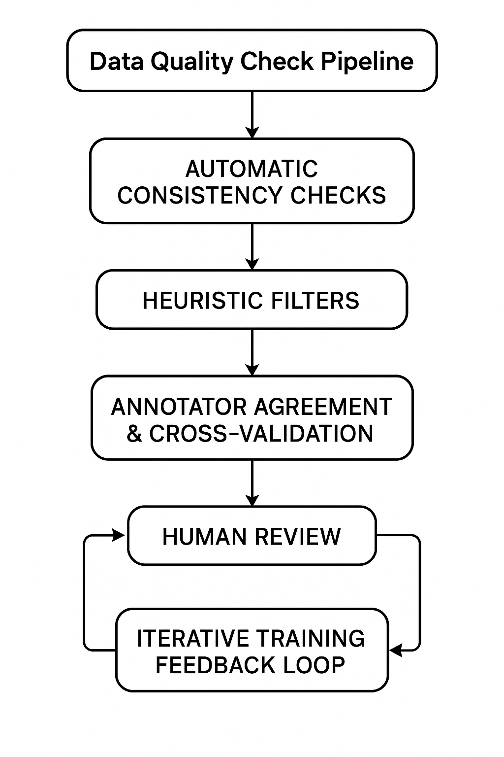
Figure 5. Data quality check pipeline.

Often one or more powerful LLMs are used in the loop as judges to identify various types of issues. Here is a checklist of common issues to look for in an SFT dataset (these can all be identified with a combination of LLM judges, code/external tools, as well as other classifiers).

Dimension	Expectation
Correctness	Every answer must be factually accurate, logically sound, and consistent with the prompt
Consistency	Style, formatting, and reasoning structure should be uniform across examples.
Completeness	Responses should fully solve the task, not just give a partial or shortcut answer.
Clarity	No unnecessary tangents, filler text, or contradictory reasoning steps.
Coverage	Dataset spans different domains, complexities, and reasoning depths, not just a single narrow slice.
Verifiability	Whenever possible, outputs should be checkable (math can be recomputed, code can be executed, reasoning can be followed).
Balance	Mix of short/simple tasks and long/complex tasks, so the model doesn’t overfit to one format.
Alignment	Outputs reflect the desired tone (helpful, concise, safe), especially important when preparing for RLHF.

How SFT Data Is Batched and Padded

Once we’ve collected instruction–response pairs for SFT, the next challenge is feeding them into the GPU efficiently. Language models work on fixed-shaped tensors: every example in a batch must be the same length [19]. But real text varies a lot — one answer might be 12 tokens, another 240 tokens. To handle this, we pack data into batches and use padding (and a fixed max sequence length T) [19, 18]; many large-scale training recipes also concatenate shorter examples and then split into fixed-length sequences to reduce padding [18, 20].

Batching means grouping several examples together so they can be processed in parallel. For instance, a batch size of 16 means the model sees 16 prompts + responses at once. This improves GPU utilization and stabilizes gradients [21]. But since sequences vary in length, we take the longest example in that batch and make every other sequence match it [20].

That’s where padding comes in. Padding tokens are special “empty” tokens (usually

PAD

) appended to shorter sequences so that all sequences in a batch share the same length [20]. The model is told to ignore these pads via an attention mask, so they don’t affect the loss [22]. Concretely:Example 1:

[The, cat, sat]

→ length 3Example 2:

[Dogs, bark, loudly, at, night]

→ length 5If batched together, we pad Example 1 to length 5:

[The, cat, sat, PAD, PAD]

In training, the attention mask is

[1, 1, 1, 0, 0]

so the loss is only computed on real tokens. This keeps gradients correct while still making tensors rectangular.

In practice, batching and padding strategies can dramatically affect throughput.

Dynamic batching (bucketing): Group examples of similar lengths together so less padding is needed.

Packed sequences: Concatenate multiple shorter examples into one long sequence, separated by special tokens, to reduce wasted space.

Masking: Ensure only “real” tokens contribute to gradients.

SFT Loss Function - Negative Log Likelihood Function

Since SFT is just a multi-class (

number of classes = vocab_size

) classification problem, the loss function used to train the model is just the negative log-likelihood (NLL) of producing the correct sequence

, given input

[13]. This is often implemented as cross-entropy between the predicted class by the model and the true class in the dataset (done at each output token sequence) [13, 1].

Mathematically, it is the following expression.

\mathcal{L}_{SFT}(\theta) = -\mathbb{E}_{(x, y) \sim \mathcal{D}} \sum_{t=1}^T \log p_{\theta} (y_t | x, y_{< t})

where,

$\theta$ are the model parameters $y_t$ is the $t$ -th token in the target response $y_{<t}$ is the prefix (previous tokens) $p_\theta(\cdot)$ is the probability distribution from the modelIn practice, this is implemented as the cross-entropy function [13, 22]. At sequence step $t$ , let $y_t^*$ denote the correct token (ground-truth dataset). Let $\log p_{\theta}(y_t^* | x, y_{<t})$ denote the log-probability of producing the token $y_t^*$ by a model with parameters $\theta$ . Then the model optimizes the function [13] $$ \mathcal{L}{SFT}(\theta) = - \frac{1}{T} \sum{t=1}^T \log p_{\theta}(y_t^* | x, y_{<t}) $$

Numerical Stability

Often for numerical stability, this function is implemented with respect to the logits of the final layer (the output of the final layer of the LLM, before passing it through a sigmoid function) [23]. Let $V$ be the vocabulary size and let $z_t \in \mathbb{R}^V$ denote the logits at last layer for the token $t$ in the sequence. Recall that the predicted distribution for $y_t^*$ is given by the expression [22, 23] $$ p_{\theta}(y_t^* | x, y_{<t}) = \frac{\exp(z_{t, y_t^*})}{\sum_{v=1}^V \exp(z_{t,v})} $$

Thus, the SFT loss simplifies to

\mathcal{L}_{SFT}(\theta) = - \frac{1}{T} \sum_{t=1}^T \left( z_{t, y_t^*} - \log \sum_{v=1}^V \exp(z_{t, v}) \right)

The second term is the commonly seen “log-sum-exp” term. Often this is computed in a numerically stable way (known as the “log-sum-exp” trick) as follows.

\log \sum_{v=1}^V \exp(z_{t, v}) = m + \log \sum_{v=1}^V \exp(z_{t, v}-m)

where

m = \max_{v=1}^V \exp(z_t, v)

Since, $z_{t,v} - m \leq 0$ , this ensures that $\exp(z_{t,v}-m) \leq 1$ and thus, there are no integer overflow issues. Integer underflow is safely rounded to 0, which is the expected behavior. Putting these together, the final SFT loss is $$ \mathcal{L}{SFT}(\theta) = - \frac{1}{T} \sum{t=1}^T \left( z_{t, y_t^*} - m - \log \sum_{v=1}^V \exp(z_{t, v}-m) \right) $$

Notes:

Relationship with pre-training loss: Note that this is the exact same loss-function used in the pre-training phase. Thus, the key difference is that instead of feeding raw sentences, the model is fed well-structured instruction pairs to constrain the learning to produce tokens that form question-answer format.

End of Message Special Token: The model will indefinitely continue producing responses, while the loss is clipped at

max_seq_len = T

. This means that, the model needs to be taught to produce full answer with $≤ T$ tokens. This is often done using special end of message tokens, that are appended to the ground truth answer.

Overfitting risk & Catastrophic forgetting: Since SFT datasets are typically much smaller than pre-training datasets, models can easily overfit. Additionally, aggressive fine-tuning may cause the model to lose its pre-trained general knowledge. Common mitigations include dropout, weight decay, early stopping, and smaller learning rates.

Curriculum design: The structure of training data significantly impacts performance. An effective approach is to begin with simple instructions and gradually introduce more complex, multi-turn interactions. Similarly, first smaller context datasets are introduced and slowly the context lengths of the datasets are increased (relevant for reasoning where the model needs to learn to generate longer and longer outputs to get higher correctness).

Pytorch Implementation: In pytorch,

F.cross_entropy(..)

implements the above numerically stable implementation of the SFT loss function, given

logits

and

targets

. Therefore, it does not require one to manually compute the max logits, and log-sum-exp terms.

In summary, SFT forms the foundation of post-training and is the first phase. In SFT, the math is simple, the data is everything, and the real art lies in balancing quality, efficiency, and coverage without destroying the pre-trained foundation.

In the next section, we will delve deeper into one of the main stages of post-training: Reinforcement Learning.

4. What Are the Common RL Training Techniques?

RL for post-training is likely the most complex aspect of post-training and arguably the most effective approach (today) for fine-tuning a model. In traditional RL, it can be thought of as a loop where an agent takes actions, which are sampled from a policy (model), w.r.t. the state of the environment, in order to maximize some rewards [24]. Adapting this for RL for post-training—we can treat the SFT model as a policy acting in an “environment” of prompts, define or learn a scalar reward that captures what you want (preferences, verifiable outcomes, or step-level scores), then sample–score–update the policy with KL-regularized policy gradients toward higher-reward behavior while anchoring to a reference model to prevent drift [3, 6, 25].

Note: This section heavily reused and condensed some of the key concepts from the incredible RLHF Book by Nathan Lambert [26]. Please refer to the original book if you want more details.

RL Rewards

Reward is a scalar value indicating the desirability of an action or state, usually denoted by $r$ . In LLM post-training, we will start with an SFT model (policy) π and a frozen reference $π₀$ (usually the initial SFT model). For a prompt $x$ and model output $y$ , we can define a scalar reward $r(x,y)$ that measures how desirable $y$ is. We then optimize a KL-regularized objective—i.e., apply policy-gradient updates while penalizing divergence from the reference model to prevent drift; the reward signal can reflect preferences, verifiable outcomes, or even step-level (process) scores [3, 25]. $$ \max_{\pi};\mathbb{E}{y\sim \pi(\cdot\mid x)}\big[r(x,y)\big];-;\beta,\mathrm{KL}!\left(\pi(\cdot\mid x),|,\pi{0}(\cdot\mid x)\right) $$ The equation above is to maximize the expected reward while constrained by the regularization using KL divergence, short for Kullback-Leibler (KL) divergence. In the first term, $r(x,y)$ is a response-level scalar reward computed after the full answer is generated, and $π(y|x)$ is the current policy (i.e. the model that you are training) [3]. KL divergence is a measure of the difference between two probability distributions $π$ and $π₀$, which tells us how far $π$ (current model) has drifted from $π₀$, the initial SFT model [27]. $β$ is a hyper-parameter that controls the strength of regularization [3].

There are a few different types of rewards that are effective in aligning the model and improving its capabilities. RLHF helps the model excel in general chats and align its safety/stylistic behaviors by leveraging reward models (RMs) trained from human preferences [3]. RLAIF (AI feedback)—also known as Constitutional AI proposed by Anthropic—uses an LLM together with a written “constitution” to scale supervision and generate preference signals [28]. RLVR (verifiable rewards) is a strong lever for improving math reasoning and coding by using ground-truth answers, unit tests, and code execution as precise signals [8]. Process supervision is more granular than RLVR, employing step-level rewards from a process reward model (PRM) to score intermediate steps in long-horizon tasks [25]. Lastly, rubrics-guided rewards can be computed by checking whether a model’s response satisfies explicit rubric criteria [29, 30]. There are usually multiple rubrics, so the overall reward is often an aggregation (e.g., a weighted sum/average) of the per-rubric scores [32]. In practice, modern post-training typically uses a hybrid, multi-stage recipe that blends several reward types across stages (e.g., SFT → preference optimization → RL with verifiable/rubric signals) [7].

Reward family	What the reward is	Where labels come from	Typical tasks	Pros and Cons
RLHF (human preferences)	Scalar from a pairwise reward model (RM) + KL to reference	Human comparisons on sampled outputs	General chat, safety/style alignment	Pros: robust, well-studied, broad coverage. Cons: RM drift/reward hacking, annotator bias, expensive data.
RLAIF / Constitutional-AI	RM trained on LLM-judge comparisons (guided by a constitution/rubric) + KL	AI-judged comparisons with light human spot-checks	Scalable helpfulness/harmlessness tuning	Pros: cheap to scale, fast iteration. Cons: judge bias/feedback loops, domain mismatch.
RLVR (verifiable outcomes)	Programmatic rewards (exact match, unit tests, execution) + KL	Ground-truth answers, tests, deterministic checkers	Math, code, factual QA	Pros: precise, low-noise signal; strong for reasoning. Cons: sparse rewards, exploitable graders, coverage gaps.
Process-supervised RL (PRMs)	Step-level rewards from a Process RM scoring CoT steps + KL	Human/AI step labels, heuristics, execution traces	Long-form reasoning, tool use	Pros: denser credit, improved faithfulness. Cons: costly step labels, PRM OOD brittleness.
Rubric-guided rewards	A rubric converted to a scalar via LLM-judge scores, PRM step scores, or executable checks + KL	LLM-judge rubric scoring; step annotations aligned to rubric; programmatic validators from rubric	Helpfulness/safety audits, style/format compliance, math/code if rubric is executable	Pros: aligns reward with intent, flexible across tasks. Cons: Goodharting weighted criteria, keyword/verbosity gaming, judge calibration drift.

Reward Models and Preferences

At the birth of RLHF for LLMs, the InstructGPT paper popularized training a reward model (RM) from human preference rankings—now a core component of RLHF [3, 31]. The most common RM predicts how close a candidate response is to what humans would prefer for a given prompt, learned from preference-labeled prompt–response sets [3, 33]. In other words, the RM estimates which output human labelers would prefer under stated guidelines. To collect preference data, a prompt and several model responses are sampled and labelers rank the outputs (best→worst, Figure 4); the resulting data train the RM, which then provides a scalar reward during RL fine-tuning [3, 33].

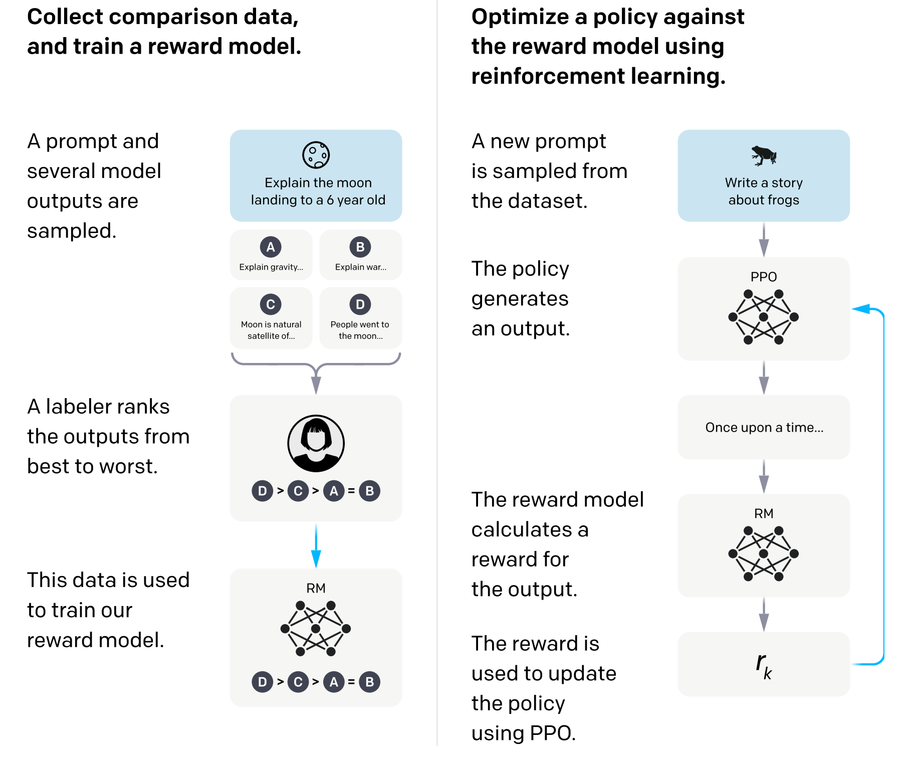
Figure 6. A Reward model (RM) training (left) and reinforcement learning via proximal policy optimization (right). This diagram is from a 2022 paper by Open AI: Training language models to follow instructions with human feedback.

What does preference data look like?

To illustrate this, let’s use the very simple example from the beginning of the doc. The simplest form of preference data involves one prompt and two responses in a pairwise fashion: a human labeler is shown a user prompt (and/or conversation history) and a pair of responses (response A, response B) sampled from a model. The job of the human labeler is to decide whether A is better than B (or vice versa) [31, 33]. This pairwise scheme can be extended to more than two responses by ranking multiple candidates or by logging decisions over arbitrary pairs, which is how many RLHF pipelines construct data for reward modeling [3, 34].

🔍 DATA EXAMPLES

User prompt:

What is the capital city of U.S.

Response A:

? The capital city of U.S. is Washington D.C.

Response B:

Washington D.C.

Figure 7. Example preference data. The job of the human label is to make a decision on whether A is better B, and if so, whether A is a lot better or just slightly better, vice versa.

JSON Format:

{ "prompt": [ {"system":"You are a helpful, honest assistant."}, {"role": "user", "content": "What color is the sky?"}, ], "chosen": [{"role": "assistant", "content": "Washington, D.C."}], "rejected": [{"role": "assistant", "content": "? The capital of the United States is Washington, D.C."}], }

In some cases, a less common method to model preference is by list-wise ranking, instead of pairwise ranking mentioned above. When there are more than two responses per prompt, list-wise ranking will assign a score to each one of the candidate responses from a pre-defined scale of scores.

Training rewards models

A standard way to train a RM is derived from the Bradley-Terry model of preference [38]. A Bradley-Terry model of preferences measures the probability that the pairwise comparison for two events drawn from the same distribution, say $i$ and $j$ , satisfy the following relation, $i >j$ : $$ P(i > j) = \frac{p_i} {p_i + p_j} $$ In the context of pairwise rewards / preferences with two samples, the $i$ and $j$ above are model completions, $y_1$ and $y_2$ , to the same prompt, $x$ . It scores both responses w.r.t a model denoted by $r_\theta$ . The success probability for a given RM in a pairwise setting becomes: $$ P(y_1 > y_2) = \frac{\exp(r(y_1))}{\exp(r(y_1)) + \exp(r(y_2)))} $$

By maximizing the log-likelihood of the above function, one can derive that the loss function now becomes:

\mathcal{L}_{pair}(\theta) = -\mathbb{E}[\log~\sigma \left(r_\theta(x, y_w) - r_\theta(x, y_l)\right)]

Now that we have decided on the loss function of the RM, we’d need to pick a backbone model to initialize the training. Usually we will be using a backbone model from the same family as the policy; a more common practice is to use the pre-trained model prior to SFT. We usually addd a scalar head (or a single linear layer / MLP) on the final token’s hidden state. RMs can also be multi-head in order to consider different dimensions and criteria separately.

For each comparison row of the preference data, it will be reformatted to be used in training:

Encode prompt:

prompt_ids = apply_chat_template(messages, add_generation_prompt=True)

.Encode answers:

chosen_ids = tok(chosen, add_special_tokens=False)

, same for

rejected