KV Caching in LLMs, Clearly Explained

文章梳理 #

本文从第一性原理出发，系统讲解了 LLM 推理中的 KV Caching 机制。

核心思路 #

LLM 自回归生成时，每一步都需要对所有 token 做 Attention 计算。其中 K（Key）和 V（Value）向量对于已生成的 token 来说是恒定不变的，但朴素实现会在每一步重新计算，造成巨大的冗余计算。KV Caching 的核心思想就是：计算一次，缓存复用。

各部分内容 #

部分	主题	要点
Part 1	Token 生成机制	Transformer 处理所有输入 token → 输出 hidden states → 投影到词表空间得到 logits → 采样得到下一个 token；只有最后一个 token 的 hidden state 有用
Part 2	Attention 计算本质	每个 token 有 Q/K/V 三个向量；最后一个 token 的 attention 只需要自己的 Q 和所有 token 的 K、V
Part 3	冗余计算问题	生成第 50 个 token 时需要 1-50 的 K/V，生成第 51 个时需要 1-51 的 K/V，而 1-49 的 K/V 完全没变却被重复计算 → 单步 O(n) 冗余，整体 O(n²) 浪费
Part 4	KV Cache 解决方案	① 只为新 token 计算 Q/K/V ② 将新 K/V 追加到缓存 ③ 从缓存读取所有历史 K/V ④ 用新 Q 对完整缓存做 Attention
Part 5	Time-to-First-Token (TTFT)	首次请求需要对整个 prompt 做 prefill（计算并缓存所有 K/V），这是计算密集阶段；缓存就绪后每步只需单 token 前向传播 → 建缓存贵，读缓存便宜
Part 6	内存 vs 计算的 Tradeoff	KV Cache 以 GPU 显存换计算速度；Qwen 2.5 72B 单请求 KV Cache 可达数 GB；因此催生了 GQA/MQA（共享 KV head 减少显存）和 Paged Attention（解决显存碎片化）

一句话总结 #

KV Caching 将 Attention 中不变的 K/V 向量缓存复用，消除自回归生成中的 O(n²) 冗余计算，实现约 5× 推理加速，代价是 GPU 显存占用——这是所有 LLM 推理引擎（vLLM、TGI、TensorRT-LLM）的基石。

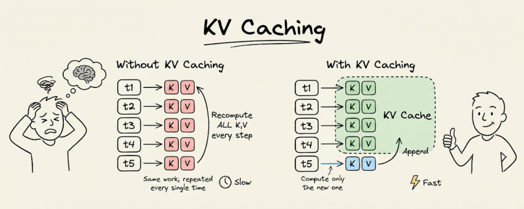
You must have seen it every time you use ChatGPT or Claude that the first token takes noticeably longer to appear. Then the rest stream out almost instantly.

Behind the scenes, it's a deliberate engineering decision called KV caching, and the purpose is to make LLM inference faster.

Before we get into the technical details, here's a side-by-side comparison of LLM inference with and without KV caching:

0:06 / 0:47

Now let's understand how it works, from first principles.

Part 1: How LLMs generate tokens #

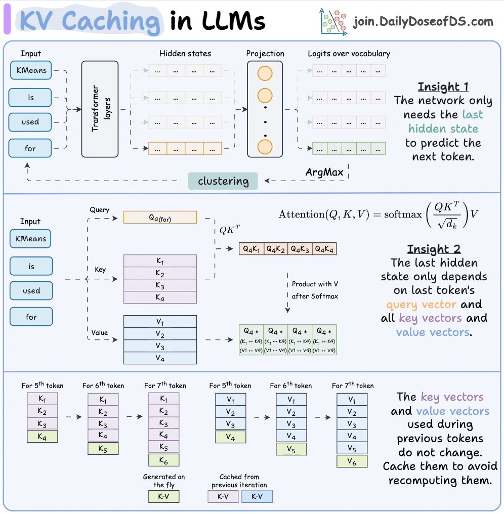
The transformer processes all input tokens and produces a hidden state for each one. Those hidden states get projected into vocabulary space, producing logits (one score per word in the vocabulary).

GIF

But only the logits from the last token matter. You sample from them, get the next token, append it to the input, and repeat.

GIF

This is the key insight: to generate the next token, you only need the hidden state of the most recent token. Every other hidden state is an intermediate byproduct.

Part 2: What Attention actually computes #

Inside each transformer layer, every token gets three vectors: a query (Q), a key (K), and a value (V). Attention multiplies queries against keys for scores, then uses those scores to weight the values.

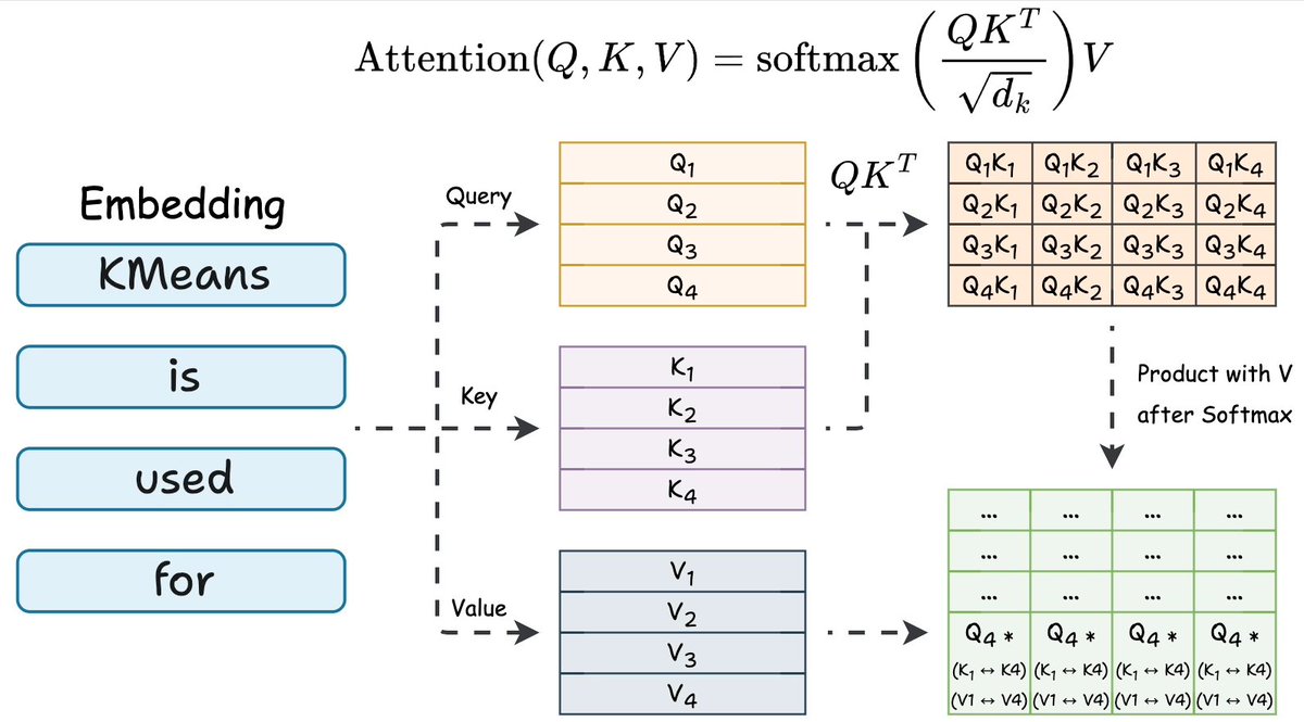
GIF

Now focus on just the last token.

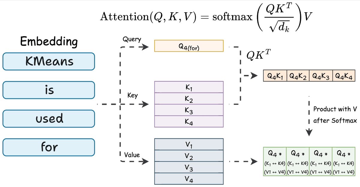
GIF

The last row of QK^T uses:

• The query vector of the last token
• All key vectors in the sequence

The final attention output for that row uses:

• The same query vector
• All key and value vectors

So to compute the only hidden state we need, every attention layer requires Q from the latest token, and K and V from everything.

Part 3: The redundancy involved #

Generating token 50 requires K and V vectors for tokens 1 through 50. Generating token 51 requires K and V vectors for tokens 1 through 51.

The K and V vectors for tokens 1 through 49 were already computed. They haven't changed. Same inputs, same outputs. Yet the model recomputes them from scratch every step.

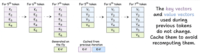
That's O(n) redundant work per step. Over an entire generation, O(n²) wasted compute.

Part 4: The fix #

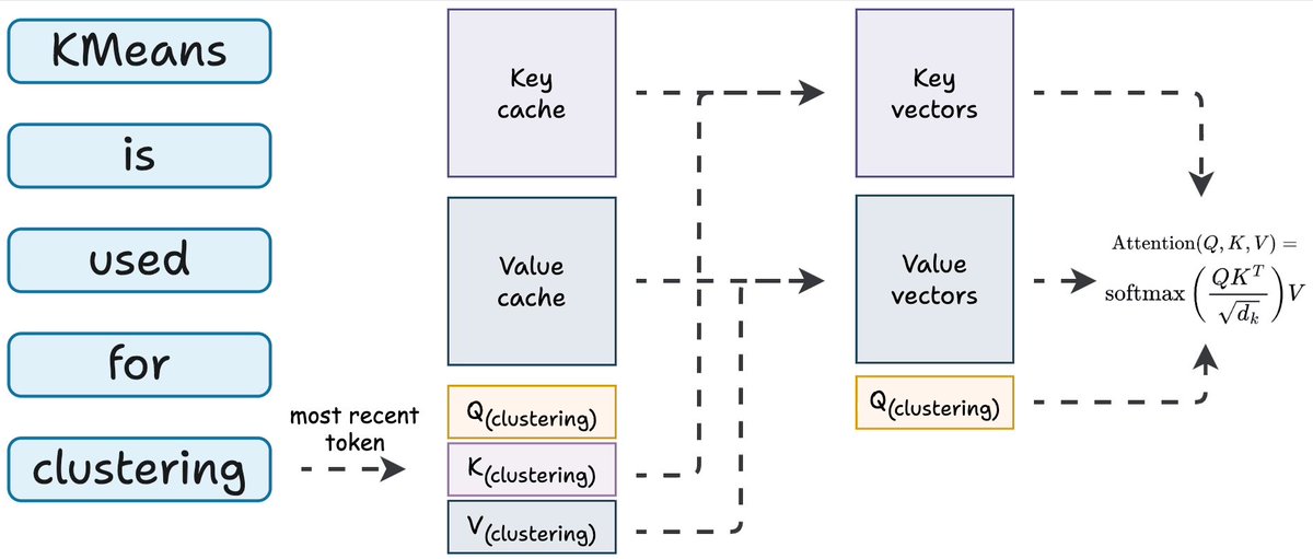
Instead of recomputing all K and V vectors at every step, store them. For each new token:

1. Compute Q, K, and V for only the newest token.
2. Append the new K and V to the cache.
3. Retrieve all previous K and V vectors from the cache.
4. Run attention using the new Q against the full cached K and V.

GIF

That's KV caching. One new K and one new V per layer per step. Everything else comes from memory.

The attention computation still scales with sequence length (you're attending over all keys and values). But the expensive projections to produce K and V happen only once per token, not once per step.

Part 5: Time-to-First-Token #

Now you can see why the first token is slow.

When you send a prompt, the model processes the entire input in one forward pass, computing and caching K and V vectors for every token. This is the prefill phase, and it's the most compute-intensive part of the request.

Once the cache is warm, each subsequent token needs only a single forward pass with one token.

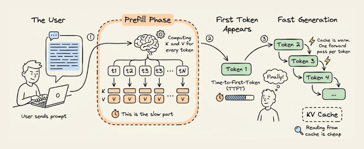
That initial delay is called time-to-first-token (TTFT). Longer prompts mean longer prefills, which mean longer waits. Optimizing TTFT (chunked prefill, speculative decoding, prompt caching) is its own deep topic, but the dynamic is always the same: building the cache is expensive, reading from it is cheap.

Part 6: The Tradeoff #

KV caching trades compute for memory. Every layer stores K and V vectors for every token. For Qwen 2.5 72B (80 layers, 32K context, hidden dim 8192), the KV cache for a single request can consume several gigabytes of GPU memory. At hundreds of concurrent requests, it often exceeds the model weights themselves.

This is why grouped-query attention (GQA) and multi-query attention (MQA) exist: share key/value heads across query heads, cut memory, and minimal quality loss.

It's also why doubling context length is hard. Double the window, double the KV cache per request, fewer concurrent users.

There is another idea called Paged attention, which solves this, and I talked about it here recently:

3月11日

tl;dr #

KV caching eliminates redundant computation during autoregressive generation. Previous tokens always produce the same K and V vectors, so you compute them once and store them. Each new token only needs its own Q, K, and V. Then, attention runs against the full cache.

5x speedup in practice. The cost is GPU memory, which becomes the binding constraint at scale. Every LLM serving stack (vLLM, TGI, TensorRT-LLM) builds on this idea.

GIF

That's a wrap!

If you enjoyed this tutorial:

Find me → @_avichawla

Every day, I share tutorials and insights on DS, ML, LLMs, and RAGs.